Quantization

Quantization is the process of representing values with a reduced number of bits. In neural networks, this corresponds to weights, activations and gradient values. Typically, when training on the GPU, values are stored in 32-bit floating point (FP) single precision. \textit{Half-precision} for floating point (FP-16) and integer arithmetic (INT-16) are also commonly considered. INT-16 provides higher precision but a lower dynamic range compared to FP-16. In FP-16, the result of a multiplication is accumulated into a FP-32 followed by a down-conversion to return to FP-16. To speed up training , faster inference and reduce bandwidth memory requirements, ongoing research has focused on training and performing inference with lower-precision networks using integer precision (IP) as low as INT-8 INT-4, INT-2 or 1 bit representations~\citep{dally2015high}. Designing such networks makes it easier to train such networks on CPUs, FPGAs, ASICs and GPUs. In practice, this often requires the storage of hidden layer outputs with full-precision (or at least with represented with more bits than the lower resolution copies). The main forward-pass and backpropogation is carried out with lower resolution copies and convert back to the full-precision stored ``accumulators'' for the gradient updates.

In the extreme case where binary weights (-1, 1) or 2-bit ternary weights (-1, 0, 1) are used in fully-connected or convolutional layers, multiplications are not used, only additions and subtractions. For binary activations, bitwise operations are used~\citep{rastegari2016xnor} and therefore addition is not used. For example, ~\citet{rastegari2016xnor} proposed XNOR-Networks, where binary operations are used in a network made up of xnor gates which approximate convolutions leading to 58 times speedup and 32 times memory savings.

##Approximating High Resolution Computation}

% quant from fp32 -> Int8 Quantizing from FP-32 to 8-bit integers with retraining can result in an unacceptable drop in performance. Retraining quantized networks has shown to be effective for maintaining accuracy in some works~\citep{gysel2018ristretto}. Other work~\citep{dettmers2015} compress gradients and activations from FP-32 to 8 bit approximations to maximize bandwidth use and find that performance is maintained on MNIST, CIFAR10 and ImageNet when parallelizing both model and data.

The quantization ranges can be found using k-means quantization~\citep{lloyd1982least}, product quantization~\citep{jegou2010product} and residual quantization~\citep{buzo1980speech}. Fixed point quantization with optimized bit width can reduce existing networks significantly without reducing performance and even improve over the original network with retraining~\citep{lin2016fixed}.

~\citet{courbariaux2014training} instead scale using shifts, eliminating the necessity of floating point operations for scaling. This involves an integer or fixed point multiplication, as apart of a dot product, followed by the shift.

~\citet{dettmers2015} have also used FP-32 scaling factors for INT-8 weights and where the scaling factor is adapted during training along with the activation output range. They also consider not adapting the min-max ranges online and clip outlying values that may occur as a a result of this in order to drastically reduce the min-max range. They find SoTA speedups for CNN parallelism, achieving a 50 time speedup over baselines on 96 GPUs.

~\citet{gupta2015deep} show that stochastic rounding techniques are important for FP-16 DNNs to converge and maintain test accuracy compared to their FP-32 counterpart models. In stochastic rounding the weight $x$ is rounded to the nearest target fixed point representation $[x]$ with probability $1 - (x - [x])/\epsilon$ where $\epsilon$ is the smallest positive number representable in the fixed-point format, otherwise $x$ is rounded to $x + \epsilon$. Hence, if $x$ is close to $[x]$ then the probability is higher of being assigned $[x]$.~\citet{wang2018training} train DNNs with FP-8 while using FP-16 chunk-based accumulations with the aforementioned stochastic rounding hardware. The necessity of stochastic rounding, and other requirements such as loss scaling, has been avoided using customized formats such as Brain float point~\citep[(BFP)][]{kalamkar2019study} which use FP-16 with the same number of exponent bits as FP-32. ~\citet{cambier2020shifted} recently propose a shifted and squeezed 8-bit FP format (S2FP-8) to also avoid the need of stochastic rounding and loss scaling, while providing dynamic ranges for gradients, weights and activations. Unlike other related 8-bit techniques ~\citep{mellempudi2019mixed}, the first and last layer do not need to be in FP32 format, although the accmulator converts the outputs to FP32.

##Adaptive Ranges and Clipping} ~\citet{park2018value} exploit the fact that most the weight and activation values are scattered around a narrower region while larger values outside such region can be represented with higher precision. The distribution is demonstrated in \autoref{fig:quant_weight_dist}, which displays the weight distribution for the $2^{nd}$ layer in the LeNet CNN network. Instead of using linear quantization shown in (c), a smaller bit interval is used for the region of where most values lie (d), leading to less quantization errors.

They propose 3-bit activations for training quantized ResNet and Inception CNN architectures during retraining. For inference on this retrained low precision trained network, weights are also quantized to 4-bits for inference with 1\% of the network being 16-bit scaling factor scalars, achieving accuracy within 1\% of the original network. This was also shown to be effective in LSTM network on language modelling, achieving similar perplexities for bitwidths of 2, 3 and 4.

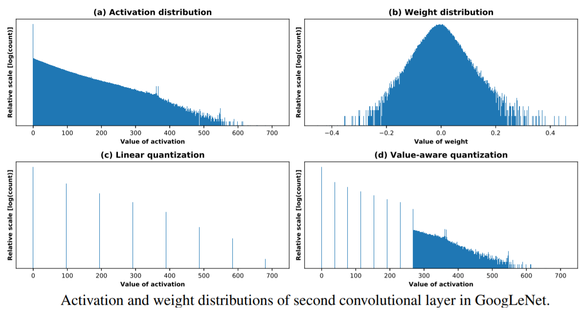
~\citet{migacz2017} use relative entropy to measure the loss of information between two encodings and aim minimize the KL divergence between activation output values. For each layer they store histgrams of activations, generate quantized distributions with different saturation thresholds and choose the threshold that minimizes the KL divergence between the original distribution and the quantized distribution.

~\citet{banner2018aciq} analyze the tradeoff between quantization noise and clipping distortion and derive an expression for the mean-squared error degradation due to clipping. Optimizing for this results in choosing clipping values that improve 40\% accuracy over standard quantization of VGG16-BN to 4-bit integer.

Another approach is to use scaling factors per group of weights (e.g channels in the case of CNNs or internal gates in LSTMs) as opposed to whole layers, particularly useful when the variance in weight distribution between the weight groupings is relatively high.

##Robustness to Quantization and Related Distortions}

~\citet{merolla2016deep} have studied the effects of different distortions on the weights and activations, including quantization, multiplicative noise (aking to Gaussian DropConnect), binarization (sign) along with other nonlinear projections and simply clipping the weights. This suggests that neural networks are robust to such distortions at the expense of longer convergence times.

% \autoref{tab:proj} shows the set of projections they consider and if they are used at training time or just applied at test time after normal FP-32 training. Here $w_{ki}$ is the i-th element of a tensor in the $k$-th layer, $\alpha_k$ normalizes the k-th layer in [-1, 1] required for some projections.

In the best case of these distortions, they can achieve 11\% test error on CIFAR-10 with 0.68 effective bits per weight. They find that training with weight projections other than quantization performs relatively well on ImageNet and CIFAR-10, particularly their proposed stochastic projection rule that leads to 7.64\% error on CIFAR-10. Others have also shown DNNs robustness to training binary and ternary networks~\citep{gupta2015deep,courbariaux2014training}, albeit a larger number of bit weight and ternary weights that are required.

##Retraining Quantized Networks} Thus far, these post-training quantization (PTQ) methods without retraining are mostly effective on overparameterized models. For smaller models that are already restricted by the degrees of freedom, PTQ can lead to relatively large performance degradation in comparison to the overparameterized regime, which has been reflected in recent findings that architectures such as MobileNet suffer when using PTQ to 8-bit integer formats and lower~\citep{jacob2018quantization,krishnamoorthi2018quantizing}.

Hence, retraining is particularly important as the number of bits used for representation decreases e.g 4-bits with range [-8, 8]. However, quantization results in discontinuities which makes differentiation during backpropogation difficult.

To overcome this limitation,~\citet{zhou2016dorefa} quantized gradients to 6-bit number and stochastically propogate back through CNN architectures such as AlexNet using straight through estimators, defined as \autoref{eq:ste_quant}. Here, a real number input $r_i \in [0, 1]$ to a n-bit number output $r_o \in [0, 1]$ and $\mathcal{L}$ is the objective function.

\begin{gather}\label{eq:ste_quant} \textbf{\text{Forward}}: r_o = \frac{1}{2^n - 1} \text{round}((2n - 1)r_i)
\textbf{\text{Backward}}: \frac{\partial \mathcal{L}}{\partial r_i} = \frac{\partial \mathcal{L}}{\partial r_o} \end{gather}

To compute the integer dot product of $r_0$ with another $n-bit$ vector, they use \autoref{eq:int_dp}, with a computational complexity of $\mathcal{O}(MK)$, directly proportional to bitwidth of $x$ and $y$. Furthermore, bitwise kernels can also be used for faster training and inference

\begin{gather}\label{eq:int_dp} x \cdot y = \sum_{m=0}^{M-1} \sum_{k=0}^{K-1}2^{m+k} \text{bitcount}[\text{and}(c_m(\vec{x}), c_k(\vec{y}))]
c_m(\vec{x})i, c_k(\vec{y}) \quad i \in {0, 1} \quad \forall i, m, k \end{gather}

####Model Distilled Quantization

An overview of our incremental network quantization method. (a) Pre-trained full precision model used as a reference. (b) Model update with three proposed operations: weight partition, group-wise quantization (green connections) and re-training (blue connections). (c) Final low-precision model with all the weights constrained to be either powers of two or zero. In the figure, operation (1) represents a single run of (b), and operation (2) denotes the procedure of repeating operation (1) on the latest re-trained weight group until all the non-zero weights are quantized. Our method does not lead to accuracy loss when using 5-bit, 4-bit and even 3-bit approximations in network quantization. For better visualization, here we just use a 3-layer fully connected network as an illustrative example, and the newly re-trained weights are divided into two disjoint groups of the same size at each run of operation (1) except the last run which only performs quantization on the re-trained floating-point weights occupying 12.5\% of the model weights.

~\citet{polino2018model} use a distillation loss with respect to the teacher network whose weights are quantized to set number of levels and quantized teacher trains the `student'. They also propose differentiable quantization, which optimizes the location of quantization points through stochastic gradient descent, to better fit the behavior of the teacher model.

%~\citet{polino2018model} propose compressing networks, referred to as `teachers', into smaller networks called students' (equivalent to Apprentice in the \citep{mishra2017apprentice} work) by using quantized distillation - a method that uses a distillation loss with respect to the teacher network whose weights are quantized to set number of levels and quantized teacher trains the student'. They also propose differentiable quantization, which optimizes the location of quantization points through stochastic gradient descent, to better fit the behavior of the teacher model.

Quantizing Unbounded Activation Functions

When the nonlinear activation unit used is not bounded in a given range, it is difficult to choose the bit range. Unlike sigmoid and tanh functions that are bounded in $[0, 1]$ and $[-1, 1]$ respectively, the ReLU function is unbounded in $[0, \infty]$. Obviously, simply avoiding such unbounded functions is one option, another is to clip values outside an upper bound~\citep{zhou2016dorefa,mishra2017wrpn} or dynamically update the clipping threshold for each layer and set the scaling factor for quantization accordingly~\citep{choi2018pact}.

Mixed Precision Training

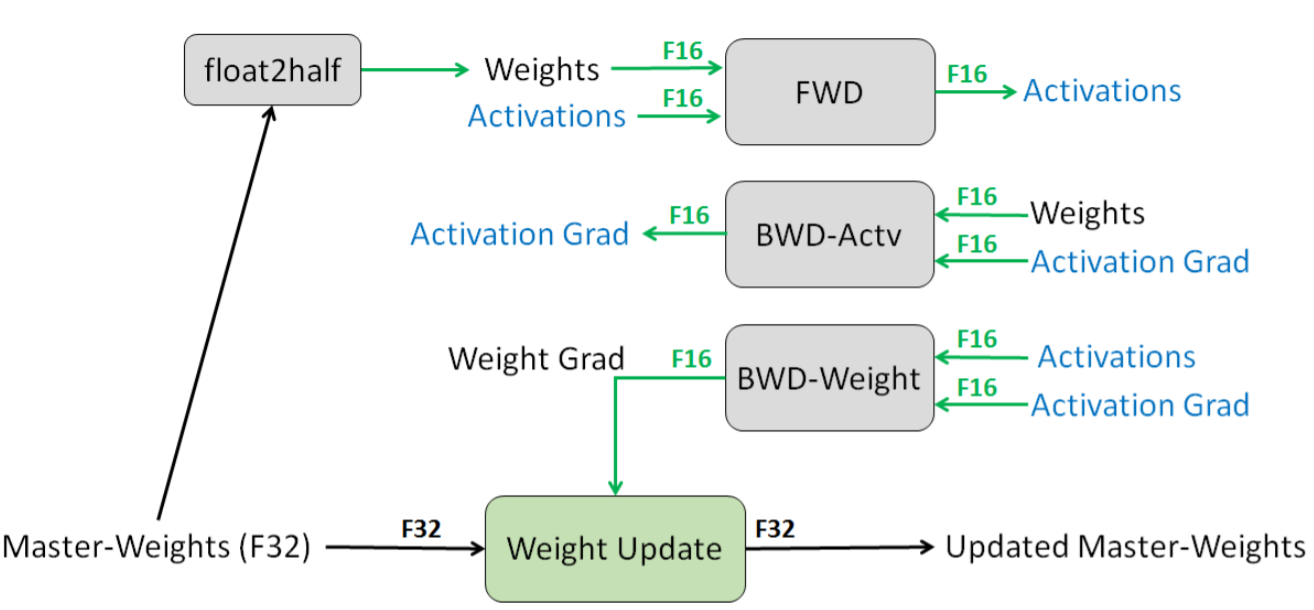
Mixed Precision Training (MPT) is often used to train quantized networks, whereby some values remain in full-precision so that performance is maintained and some of the aforementioned problems (e.g overflows) do not cause divergent training. It has also been observed that activations are more sensitive to quantization than weights~\citep{zhou2016dorefa}

~\citet{micikevicius2017mixed} use half-precision (16-bit) floating point accuracy to represent weights, activations and gradients, without losing model accuracy or having to modify hyperparameters, almost halving the memory requirements. They round a single-precision copy of the weights for forward and backward passes after performing gradient-updates, use loss-scaling to preserve small magnitude gradient values and perform half-precision computation that accumulates into single-precision outputs before storing again as half-precision in memory.

~\autoref{fig:mpt} illustrates MPT, where the forward and backward passes are performed with FP-16 precision copies. Once the backward pass is performed the computed FP-16 gradients are used to update the original FP-32 precision master weight. After training, the quantized weights are used for inference along with quantized activation units. This can be used in any type of layer, convolutional or fully-connected.

Others have focused solely on quantizing weights, keeping the activations at FP32 ~\citep{li2016ternary,zhu2016trained}.During gradient descent,~\citet{zhu2016trained} learn both the quantized ternary weights and pick which of these values is assigned to each weight, represented in a codebook.

Loss Scaling & Stochastic Rounding

~\citet{das2018mixed} propose using Integer Fused-Multiply-and-Accumulate (FMA) operations to accumulate results of multiplied INT-16 values into INT-32 outputs and use dynamic fixed point scheme to use in tensor operations. This involves the use of a shared tensor-wide exponent and down-conversion on the maximum value of an output tensor at each given training iteration using stochastic, nearest and biased rounding. They also deal with overflow by proposing a scheme that accumulates INT-32 intermediate results to FP-32 and can trade off between precision and length of the accumulate chain to improve accuracy on the image classification tasks. They argue that previous reported results on mixed-precision integer training report on non-SoTA architectures and less difficult image tasks and hence they also report their technique on SoTA architectures for the ImageNet 1K dataset.

Quantizing by Adapting the Network Structure}

To further improve over mixed-precision training, there has been recent work that have aimed at better simulating the effects of quantization during training.

~\citet{mishra2017apprentice} combine low bit precision and knowledge distillation using three different schemes: (1) a low-precision (4-bit) ResNet network is trained from a full-precision ResNet network both from scratch, (2) a full precision trained network is transferred to train a low-precision network from scratch and (3) a trained full-precision network guides a smaller full-precision student randomly initialized network which is gradually becomes lower precision throughout training. They find that (2) converges faster when supervised by an already trained network and (3) outperforms (1) and set at that time was SoTA for Resnet classifiers at ternary and 4-bit precision.
~\citet{lin2017towards} replace FP-32 convolutions with multiple binary convolutions with various scaling factors for each convolution, overall resulting in a large range.

~\citet{zhou2016dorefa} and~\citet{choi2018pact} have both reported that the first and last convolutional layers are most sensitive to quantization and hence many works have avoided quantization on such layers. However,~\citet{choi2018pact} find that if the quantization is not very low (e.g 8-bit integers) then these layers are expressive enough to maintain accuracy.

~\citet{zhou2017incremental} have overcome this problem by iteratively quantizing the network instead of quantize the whole model at once. During the retraining of an FP-32 model, each layer is iteratively quantized over consecutive epochs. They also consider using supervision from a teacher network to learn a smaller quantized student network, combining knowledge distillation with quantization for further reductions.

Quantization with Pruning & Huffman Coding

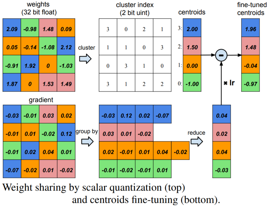
Coding schemes can be used to encode information in an efficient manner and construct codebooks that represent weight values and activation bit spacing.~\citet{han2015deep} use pruning with quantization and huffman encoding for compression of ANNs by 35-49 times (9-13 times for pruning, quantization represents the weights in 5 bits instead of 32) the original size without affecting accuracy.

Once the pruned network is established, the parameter are quantized to promote parameter sharing. This multi-stage compression strategy is illustrated in \autoref{fig:sqft}, showing the combination of weight sharing (top) and fine-tuning of centroids (bottom). They note that too much pruning on channel level sparsity (as opposed to kernel-level) can effect the network's representational capacity.

Loss-aware quantization

~\citet{hou2016loss} propose a proximal Newton algorithm with a diagonal Hessian approximation to minimize the loss with respect to the binarized weights \(\hat{\vec{w}} = \alpha \vec{b}\), where \(\alpha > 0\) and \(\vec{b}\) is binary. During training, \(\alpha\) is computed for the \(l\)-th layer at the \(t\)-th iteration as \(\alpha^t_l = || \vec{d}^{t - 1} \otimes \vec{w}^t_l ||_1 / || \vec{d}^{t - 1 }_l ||_1\) where \(\vec{d}^{t - 1}_l := \text{diag}(\mathbf{D}^{t - 1}_{l})\) and \(\vec{b}^{t}_l = \sign(\vec{w}^t_l)\). The input is then rescaled for layer $l$ as $\tilde{\vec{x}}^t_l = \alpha^t_l \vec{x}^t_{l-1}$ and then compute $\vec{z}^t_l$ with input $\tilde{x}^t_{l-1}$ and binary weight $\vec{b}^{t}_l$.

~\autoref{eq:proximal_newton} shows the proximal newton update step where $w^{t}_{l}$ is the weight update at iteration $t$ for layer $l$, $\mathbf{D}$ is an approximation to the diagonal of the Hessian which is already given as the $2^{nd}$ momentum of the adaptive momentum (adam) optimizer. The $t$-th iteration of the proximal Newton update is as follows:

where the loss \(\ell\) w.r.t binarized version of \(\ell(w_t)\) is expressed in terms of the \(2^{nd}\)-order TS expansion using a diagonal approximation of the Hessian \(\mathbf{H}^{t-1}\), which estimates of the Hessian at \(\vec{w}^{t-1}\). Similar to the \(2^{nd}\) order approximations discussed in~\autoref{eq:weight_reg}, the Hessian is essential since \(\ell\) is often flat in some directions but highly curved in others.

Explicit Loss-Aware Quantization

~\citet{zhou2018explicit} propose an Explicit Loss-Aware Quantization (ELQ) method that minimizes the loss perturbation from quantization in an incremental way for very low bit precision i.e binary and ternary. Since going from FP-32 to binary or ternary bit representations can cause considerable fluctuations in weight magnitudes and in turn the predictions, ELQ directly incorporates this quantization effect in the loss function as

where \(L_p\) is the loss difference between quantized and the original model \(||\mathcal{L}(\mathbf{W}_l) - \mathcal{L}(\hat{\mathbf{W}}_l)||\), \(E\) is the reconstruction error between the quantized and original weights \(||\mathbf{W}_l - \hat{\mathbf{W}_l}||^2\), \(a_l\) a regularization coefficient for the \(l\)-th layer and \(c_k\) is an integer and $k$ is the number of weight centroids.

Value-aware quantization

~\citet{park2018value} like prior work mentioned in this work have also succeeded in reduced precision by reducing the dynamic range by narrowing the range where most of the weight values concentrate. Different to other work, they assign higher precision to the outliers as opposed to mapping them to the extremum of the reduced range. This small difference allow 3-bit activations to be used in ResNet-152 and DenseNet-201, leading to a 41.6\% and 53.7\% reduction in network size respectively.

Differentiable Quantization

When considering fully-differentiable training with quantized weight and activations, it is not obvious how to back-propagate through the quantization functions. These functions are discrete-valued, hence their derivative is 0 almost everywhere. So, using their gradients as-is would severely hinder the learning process. A commonly used approximation to overcome this issue is the ``straight-through estimator'' (STE)~\citep{hinton2012neural,bengio2013estimating}, which simply passes the gradient through these functions as-is, however there has been a plethora of other techniques proposed in recent years which we describe below.

Differentiable Soft Quantization

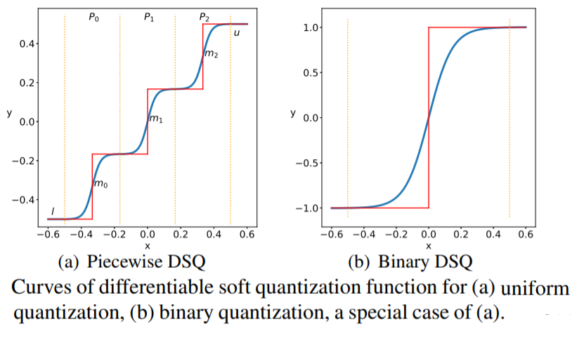
~\citet{gong2019differentiable} have proposed differentiable soft quantization (DSQ) learn clipping ranges in the forward pass and approximating gradients in the backward pass. To approximate the derivative of a binary quantization function, they propose a differentiable asymptotic function (i.e smooth) which is closer to the quantization function that it is to a full-precision $\mathtt{tanh}$ function and therefore will result in less of a degradation in accuracy when converted to the binary quantization function post-training.

For multi-bit uniform quantization, given the bit width $b$ and the floating-point activation/weight \(\vec{x}\) following in the range \((l, u)\), the complete quantization-dequantization process of uniform quantization can be defined as: \(Q_U(\vec{x}) = \text{round}(\vec{x} \Delta)\Delta$ where the original range $(l, u)\) is divided into \(2^b - 1\) intervals \(\mathcal{P}_i, i \in (0, 1, \ldots 2^b - 1)\), and \(\Delta = \frac{u-l}{2^b-1}\) is the interval length.

The DSQ function, shown in \autoref{eq:soft_quant_tanh}, handles the point \(\vec{x}\) depending what interval in \(\mathcal{P}_i\) lies.

with

The scale parameter $s$ for the tanh function \(\varphi\) ensures a smooth transitions between adjacent bit values, while \(k\) defines the functions shape where large \(k\) corresponds close to consequtive step functions given by uniform quantization with multiple piecewise levels, as shown in \autoref{fig:diff_soft_quant}. The DSQ function then approximates the uniform quantizer \(\varphi\) as follows:

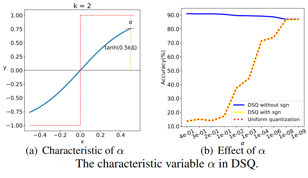
The DSQ can be viewed as aligning the data with the quantization values with minimal quantization error due to the bit spacing that is carried out to reflect the weight and activation distributions. \autoref{fig:dsq} shows the DSQ curve without [-1, 1] scaling, noting standard quantization is near perfectly approximated when the largest value on the curve bounded by +1 is small. They introduce a characteristic variable $\alpha: = 1 - \tanh(0.5 k \Delta) = 1 - \frac{1}{s}$ and given that,

\begin{gather} \Delta = \frac{u-l}{2^b - 1}
\varphi(0.5\Delta) = 1 \quad \Rightarrow \quad k = \frac{1}{\Delta}\log( 2/\alpha - 1) \end{gather}

DSQ can be used as a piecewise uniform quantizer and when only one interval is used, it is the equivalent of using DSQ for binarization.

Soft-to-hard vector quantization

~\citet{agustsson2017soft} propose to compress both the feature representations and the model by gradually transitioning from soft to hard quantization during retraining and is end-to-end differentiable. They jointly learn the quantization levels with the weights and show that vector quantization can be improved over scalar quantization.

They optimize the rate distortion trade-off between the expected loss and the entropy of \(\mathbb{E}(Z)\):

####Iterative Product Quantization (iPQ)} Quantizing a whole network at once can be too severe for low precision (< 8 bits) and can lead to \textit{quantization drift} - when scalar or vector quantization leads to an accumulation of reconstruction errors within the network that compound and lead to large performance degradations. To combat this, ~\citet{stock2019and} iteratively quantize the network starting with low layers and only performing gradient updates on the rest of the remaining layers until they are robust to the quantized layers. This is repeated until quantization is carried out on the last layer, resulting in the whole network being amenable to quantization. The codebook is updated by averaging the gradients of the weights within the block \(b_{\text{KL}}\) as

where \(\mathcal{L}\) is the loss function, \(I_{\text{KL}}\) is an index for the \((k, l)\) subvector and \(\eta > 0\) is the codebook learning rate. This adapts the upper layers to the drift appearing in their inputs, reducing the impact of the quantization approximation on the overall performance.

Quantization-Aware Training

Instead of iPQ,~\citet{jacob2018quantization} use a straight through estimator ~\citep[(STE)][]{bengio2013estimating} to backpropogate through quantized weights and activations of convolutional layers during training.~\autoref{fig:iaoq} shows the 8-bit weights and activations, while the accumulator is represented in 32-bit integer.

They also note that in order to have a challenging architecture to compress, experiments should move towards trying to compress architectures which are already have a minimal number of parameter and perform relatively well to much larger predecessing architectures e.g EfficientNet, SqueezeNet and ShuffleNet.

Quantization Noise

~\citet{fan2020training} argue that both iPQ and QAT are less suitable for very low precision such as INT4, ternary and binary. They instead propose to randomly simulate quantization noise on a subset of the network and only perform backward passes on the remaining weights in the network. Essentially this is a combination of DropConnect (instead of the Bernoulli function, it is a quantization noise function) and Straight Through Estimation is used to backpropogate through the sample of subvectors chosen for quantization for a given mini-batch.

Estimating quantization noise through randomly sampling blocks of weights to be quantized allows the model to become robust to very low precision quantization without being too severe, as is the case with previous quantization-aware training~\citep{jacob2018quantization}. The authors show that this iterative quantization approach allows large compression rates in comparison to QAT while staying close to (few perplexity points in the case of language modelling and accuracy for image classification) the uncompressed model in terms of performance. They reach SoTA compression and accuracy tradeoffs for language modelling (compression of Transformers such as RoBERTa on WikiText) and image classification (compressing EfficientNet-B3 by 80\% on ImageNet).

####Hessian-Based Quantization The precision and order (by layer) of quantization has been chosen using $2^{nd}$ order information from the Hessian~\citep{dong2019hawq}. They show that on already relatively small CNNs (ResNet20, Inception-V3, SqueezeNext) that Hessian Aware Quantization (HAWQ) training leads to SoTA compression on CIFAR-10 and ImageNet with a compression ratio of 8 and in some cases exceed the accuracy of the original network with no quantization.

Similarly,~\citet{shen2019q} quantize transformer-based models such as BERT with mixed precision by also using $2^{nd}$ order information from the Hessian matrix. They show that each layer exhibits varying amount of information and use a sensitivity measure based on mean and variance of the top eigenvalues. They show the loss landscape as the two most dominant eigenvectors of the Hessian are perturbed and suggest that layers that shower a smoother curvature can undergo lower but precision. In the cases of MNLI and CoNLL datasets, upper layers closer to the output show flatter curvature in comparison to lower layers. From this observation, they are motivated to perform a group-wise quantization scheme whereby blocks of a matrix have different amounts of quantization with unique quantization ranges and look up table. A Hessian-based mixed precision scheme is then used to decide which blocks of each matrix are assigned the corresponding low-bit precisions of varying ranges and analyse the differences found for quantizing different parts of the self-attention block (self-attention matrices and fully-connected feedforward layers) and their inputs (embeddings) and find the highest compression ratios can be attributed to most of the parameters in the self-attention blocks.