Knowledge Distillation

Knowledge distillation involves learning a smaller network from a large network using supervision from the larger network and minimizing the entropy, distance or divergence between their probabilistic estimates.

To our knowledge,~\citet{bucilua2006model} first explored the idea of reducing model size by learning a student network from an ensemble of models. They use a teacher network to label a large amount of unlabeled data and train a student network using supervision from the pseudo labels provided by the teacher. They find performance is close to the original ensemble with 1000 times smaller network.

~\citet{hinton2015distilling} a neural network knowledge distillation approach where a relatively small model (2-hidden layer with 800 hidden units and ReLU activations) is trained using supervision (class probability outputs) for the original ``teacher'' model (2-hidden layer, 1200 hidden units). They showed that learning from the larger network outperformed the smaller network learning from scratch in the standard supervised classification setup. In the case of learning from ensemble, the average class probability is used as the target.

The cross entropy loss is used between the class probability outputs of the student output \(y^S\) and one-hot target $y$ and a second term is used to ensure that the student representation \(z^s\) is similar to the teacher output $z^T$. This is expressed in terms of KL divergence as,

The idea of training a student network on the logit outputs (i.e log of the predicted probabilities) of the teacher to gain more information from the teacher network can be attributed to the work of~\citet{ba2014deep}. By using logits, as opposed to a softmax normalization across class probabilities for example, the student network better learns the relationship between each class on a log-scale which is more forgiving than the softmax when the differences in probabilities are large.

%~\citet{bucilua2006model} showed that ensembles, referred to as a \textit{mixture of experts}, can be compressed into a single model that could reach the same performance as the original ensemble.

% In traditional knowledge distillation [12], the softened class scores of the teacher are used as the extra supervisory signal: the distillation loss encourages the student to mimic the scores of the teacher.

\subsection{Analysis of Model Distillation} The works in this subsection provide insight into the relationship between the student and teacher networks for various tasks, teacher size and network size. We also discuss work that focuses on what is required to train a well-performing student network e.g use of early stopping~\citep{tarvainen2017mean} and avoiding training the teacher network with label smoothing~\citep{muller2019does}.

\paragraph{Theories of Why Knowledge Distillation Works} %Training a student network from the soft outputs of the teacher network~\citep{hinton2015distilling}

For a distilled linear classifier, ~\citet{phuong2019towards} prove a generalization bound that shows the fast convergence of the expected loss. In the case where the number of samples is less than the dimensionality of the feature space, the weights learned by the student network are projections of the weights in the student network onto the data span. Since gradient descent makes updates that are within the data space, the student network is bounded in this space and therefore it is the best student network can approximate of the teacher network weights w.r.t the Euclidean norm. From this proof, they identify 3 important factors that contribute that explain the success of knowledge distillation - (1) the geometry of the data distribution that makes up the separation between classes greatly effects the student networks convergence rate (2), gradient descent is biased towards a desirable minimum in the distillation objective and (3) the loss monotonically decreases proportional to size of the training set.

\paragraph{Teacher Assistant Model Distillation}

~\citet{mirzadeh2019improved} show that the performance of the student network degrades when the gap between the teacher and the student is too large for the student to learn from. Hence, they propose an intermediate `teaching assistant' network to supervise and distil the student network where the intermediate networks is distilled from the teacher network.

~\autoref{fig:distil_perf} shows their plot, where on the left side a) and b) we see that as the gap between the student and teacher networks widen when the student network size is fixed, the performance of student network gradually degrades. Similarly, on the right hand side, a similar trend is observed when the student network size is increased with a fixed teacher network.

Theoretical analysis and extensive experiments on CIFAR-10,100 and ImageNet datasets and on CNN and ResNet architectures substantiate the effectiveness of our proposed approach.

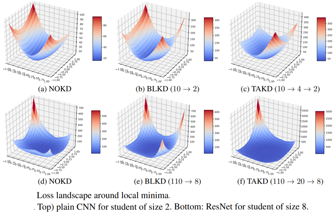
Their \autoref{fig:loss_landscape} shows the loss surface of CNNs trained on CIFAR-100 for 3 different approaches: (1) no distillation, (2) standard knowledge distillation and (3) teaching assisted knowledge distillation. As shown, the teaching assisted knowledge distillation has a smoother surface around the local minima, corresponding to more robustness when the inputs are perturbed and better generalization.

On the Efficacy of Model Distillation

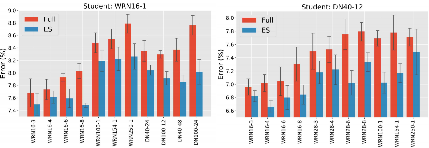
~\citet{cho2019efficacy} analyse what are some of the main factors in successfully using a teacher network to distil a student network. Their main finding is that when the gap between the student and teacher networks capacity is too large, distilling a student network that maintains performance or close to the teacher is either unattainable or difficult. They also find that the student network can perform better if early stopping is used for the teacher network, as opposed to training the teacher network to convergence. \autoref{fig:early_stop_teacher} shows that teachers (DenseNet and WideResNet) trained with early stopping are better suited as supervisors for the student network (DenseNet40-12 and WideResNet16-1).

Avoid Training the Teacher Network with Label Smoothing

~\citet{muller2019does} show that because label smoothing forces the same class sample representations to be closer to each other in the embedding space, it provides less information to student network about the boundary between each class and in turn leads to poorer generlization performance. They quantify the variation in logit predictions due to the hard targets using mutual information between the input and output logit and show that label smoothing reduces the mutual information. Hence, they draw a connection between label smoothing and information bottleneck principle and show through experiments that label smoothing can implicitly calibrate the predictions of a DNN.

Distilling with Noisy labels

~\citet{sau2016deep} propose to use noise to simulate learning from multiple teacher networks by simply adding Gaussian noise the logit outputs of the teacher network, resulting in better compression when compared to training with the original logits as targets for the teacher network. They choose a set of samples from each mini-batch with a probability $\alpha$ to perturbed by noise while the remaining samples are unchanged. They find that a relatively high $\alpha=0.8$ performed the best for image classification task, corresponding to 80\% of teacher logits having noise.

~\citet{li2017learning} distil models with noisy labels and use a small dataset with clean labels, alongside a knowledge graph that contains the label relations, to estimate risk associated with training using each noisy label. A model is trained on the clean dataset $D_c$ and the main model is trained over the whole dataset $D$ with noisy labels using the loss function,

where \(s_i=\delta[f^D_c(\vec{x}i)]\). The first loss term is cross entropy between student noisy and noisy labels and the second term is the loss between the the hard target $s_i$ given by the model trained on clean data and the model trained on noisy data.

They also use pseudo labels $\hat{y}\lambda_i= \lambda \vec{y}_i+ (1 - \lambda)\vec{s}_i$ that combine noisy label $\vec{y}_i$ with the output $\vec{s}_i$ trained on $D_c$. This motivated by the fact that both noisy label and the predicted labels from clean data are independent and this can be closer to true labels $y^{*}_i$ under conditions which they further detail in the paper.

To avoid the model trained on $D_c$ overfitting, they assign label confidence score based on related labels from a knowledge graph, resulting in a reduction in model variance during knowledge distillation.

Distillation of Hidden Layer Activation Boundaries

Instead of transferring the outputs of the teacher network,~\citet{heo2019knowledge} transfer activation boundaries, essentially outputs which neurons are activated and those that are not. They use an activation loss that minimizes the difference between the student and teacher network activation boundaries, unlike previous work that focuses on the activation magnitude. Since gradient descent updates cannot be used on the non-differentiable loss, they propose an approximation of the activation transfer loss that can be minimized using gradient descent. The objective is given as,

where \(\mathcal{S}(\mathcal{I})$ and $\mathcal{T}(\mathcal{I})\) are the neuron response tensors for student and teacher networks, $\rho(\mathcal{T}(I))$ is the the activation of teacher neurons corresponding to class labels, $r(\mathcal{S}(\mathcal{I}))$ is the , $r$ is a connector function (a fully connected layer in their experiments) that converts a neuron response vector of student to the same size as the teacher vector, $\circ$ is elementwise product of vectors and $\mu$ is the margin to stabilize training.

Simulating Ensembled Teachers Training

~\citet{park2020improved} have extended the idea of student network learning from a noisy teacher to speech recognition and similarly found high compression rates. ~\citet{han2018co} have pointed out that co-teaching (where two networks learn from each other where one has clean outputs and the other has noisy outputs) avoids a single DNN from learning to memorize the noisy labels and select samples from each mini-batch that the networks should learn from and avoid those samples which correspond to noisy labels. Since both networks have different ways of learning, they filter different types of error occurring from the noisy labels and this information is communicated mutually. This strategy could also be useful for using the teacher network to provide samples to a smaller student network that improve the learning of the student.

Layer Fusion

Layer Fusion (LF)~\citep{neill2020compressing} is a technique to identify similar layers in very deep pretrained networks and fuse the top-k most similar layers during retraining for a target task. Various alignments measures are proposed that have desirable properties of for layer fusion and freezing, averaging and dynamic mixing of top-k layer pairs are all experimented with for fusing the layers. This can be considered as unique approach to knowledge distillation as it does aim to preserve the knowledge in the network while preserving network density, but without having to train a student network from scratch.

Distilling Recurrent (Autoregressive) Neural Networks

Although the work by ~\citet{bucilua2006model} and ~\citet{hinton2015distilling} has often proven successful for reducing the size of neural models in other non-sequential tasks, many sequential tasks in NLP and CV have high-dimensional outputs (machine translation, pixel generation, image captioning etc.). This means using the teachers probabilistic outputs as targets can be expensive. ~\citet{kim2016sequence} use the teachers hard targets (also 1-hot vectors) given by the highest scoring beam search prediction from an encoder-decoder RNN, instead of the soft output probability distribution. The teacher distribution $q(y_t|x)$ is approximated by its mode:$q(y_s|x) \approx 1{t= \operatorname{argmax}_{y_t \in \mathcal{Y}} q(y_t|x)}$ with the following objective

where \(y_t \in \mathcal{Y}\) are teacher targets (originally defined by the predictions with the highest scoring beam search) in the space of possible target sequences. When the temperature \(\tau \to 0\), this is equivalent to standard knowledge distillation.

In sequence-level interpolation, the targets from the teacher with the highest \textit{similarity} with the ground truth are used as the targets for the student network. Experiments on NMT showed performance improvements compared to soft targets and further pruning the distilled model results in a pruned student that has 13 times fewer parameters than the teacher network with a 0.4 decrease in BLEU metric.

%Our best student model runs 10 times faster than its %state-of-the-art teacher with little loss in performance. It is also significantly better than a baseline model trained without knowledge distillation: by 4.2/1.7 BLEU with greedy decoding/beam search. Applying weight pruning on top of knowledge distillation results in a student model that has 13x fewer parameters than the original teacher model, with a decrease of 0.4 BLEU.

Distilling Transformer-based (Non-Autoregressive) Networks

Knowledge distillation has also been applied to very large transformer networks, predominantly on BERT~\citep{devlin2018bert} given its wide success in NLP. Thus, there has been a lot of recent work towards reducing the size of BERT and related models using knowledge distillation.

DistilBERT

~\citet{sanh2019distilbert} achieves distillation by training a smaller BERT on very large batches using gradient accumulation, uses dynamic masking, initializes the student weights with teacher weights and removes the next sentence prediction objective. They train the smaller BERT model on the original data BERT was trained on and fine that DistilBERT is within 3\% of the original BERT accuracy while being 60\% faster when evaluated on the GLUE~\citep{wang2018glue} benchmark dataset.

BERT Patient Model Distillation

Instead of minimizing the soft probabilities between the student and teacher network outputs,~\citet{sun2019patient} propose to also learn from the intermediate layers of the BERT teacher network by minimizing the mean squared error between adjacent and normalized hidden states. This loss is combined with the original objective proposed by~\citet{hinton2015distilling} which showed further improves in distilling BERT on the GLUE benchmark datasets~\citep{wang2018glue}.

TinyBERT

TinyBERT~\citep{jiao2019tinybert} combines multiple Mean Squared Error (MSE) losses between embeddings, hidden layers, attention layers and prediction outputs between $S$ and $T$. The TinyBERT distillation objective is shown below, where it combines multiple reconstruction errors between $S$ and $T$ embeddings (when m=0), between the hidden and attention layers of $S$ and $T$ when $ M \geq m > 0$ where $M$ is index of the last hidden layer before prediction layer and lastly the cross entropy between the predictions where $t$ is the temperature of the softmax.

Through many ablations in experimentations, they find distilling the knowledge from multi-head attention layers to be an important step in improving distillation performance.

ALBERT

~\citet{lan2019albert} proposed factorized embeddings to reduce the size of the vocabulary embeddings and parameter sharing across layers to reduce the number of parameters without a performance drop and further improve performance by replacing next sentence prediction with an inter-sentence coherence loss. ALBERT is. 5.5\% the size of original BERT and has produced state of the art results on top NLP benchmarks such as GLUE~\citep{wang2018glue}, SQuAD~\citep{rajpurkar2016squad} and RACE~\citep{lai2017race}.

BERT Distillation for Text Generation

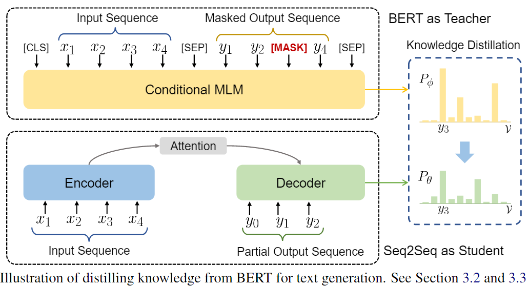
~\citet{chen2019distilling} use a conditional masked language model that enables BERT to be used on generation tasks. The outputs of a pretrained BERT teacher network are used to provide sequence-level supervision to improve Seq2Seq model and allow them to plan ahead.~\autoref{fig:bert_distil_text_gen} illustrates the process, showing where the predicted probability distribution for the remaining tokens is minimized with respect to the masked output sequence from the BERT teacher.

Applications to Machine Translation

~\citet{zhou2019understanding} seek to better understand why knowledge distillation leads to better non-autoregressive distilled models for machine translation. They find that the student network finds it easier to model variations in the output data since the teacher network reduces the complexity of the dataset.

Ensemble-based Model Distillation

Ensembles of Teacher Networks for Speech Recognition

~\citet{chebotar2016distilling} use the labels from an ensemble of teacher networks to supervise a student network trained for acoustic modelling. To choose a good ensemble, one can select an ensemble where each individual model potentially make different errors but together they provide the student with strong signal for learning. Boosting weights each sample based proportional to its misclassification rate. Similarly this can used on the ensemble to learn which outputs from each model to use for supervision. Instead of learning from a combination of teachers that are best by using an oracle that approximates the best outcome of the ensemble for automatic speech recognition (ASR) as

where the oracle \(O(u) \in 1 \ldots N\) that contains \(N\) teachers assigns all the weight to the model that has the lowest word errors for a given utterance $u$. Each model is an RNN of different architecture trained with different objectives and the student $s$ is trained using the Kullbeck Leibler (KL) divergence between oracle assigned teachers output and the student network output. They achieve an \(8.9\%\) word error rate improvement over similarly structured baseline models.

~\citet{freitag2017ensemble} apply knowledge distillation to NMT by distilling an ensemble of networks and oracle BLEU teacher network into a single NMT system. The find a student network of equal size to the teacher network outperforms the teacher after training. They also reduce training time by only updating the student networks with filtered samples based on the knowledge of the teacher network which further improves translation performance.

~\citet{cui2017knowledge} propose two strategies for learning from an ensemble of teacher network; (1) alternate between each teacher in the ensemble when assigning labels for each mini-batch and (2) simultaneously learn from multiple teacher distributions via data augmentation. They experiment on both approaches where the teacher networks are deep VGG and LSTM networks from acoustic models.

~\citet{cui2017knowledge} extend knowledge distillation to multilingual problems. They use multiple pretrained teacher LSTMs trained on multiple low-resource languages to distil into a smaller standard (fully-connected) DNN. They find that student networks with good input features makes it easier to learn from the teachers labels and can improve over the original teacher network. Moreover, from their experiments they suggest that allowing the ensemble of teachers learn from one another, the distilled model further improves.

Mean Teacher Networks

~\citet{tarvainen2017mean} find that averaging the models weights of an ensemble at each epoch is more effective than averaging label predictions for semi-supervised learning. This means the Mean Teacher can be used as unsupervised learning distillation approach as the distiller does not need labels. than methods which rely on supervision for each ensemble model. They find this straightforward approach to outperform previous ensemble based distillation approaches~\citep{laine2016temporal} when only given 1000 labels on the Street View House View Number~\citep[SVHN;][]{goodfellow2013multidig} dataset. Moreover, using Mean Teacher networks with Residual Networks achieved SoTA with 4000 labels from 10.55\% error to 6.28\% error.

on-the-fly native ensemble

~\citet{zhu2018knowledge} focus on using distillation on the fly in a scenario where the teacher may not be fully pretrained or it does not have a high capacity. This reduces compression from a two-phase (pretrain then distil) to one phase where both student and teacher network learn together. They propose an On the fly Native Ensemble (ONE) learning strategy that essentially learns a strong teacher network that assists the student network as it is learning. Performance improvements for on the fly distillation are found on the top benchmark image classification datasets.

Multi-Task Teacher Networks

~\citet{liu2019improving} perform knowledge distillation for performing multi-task learning (MTL), using the outputs of teacher models from each natural language understanding (NLU) task as supervision for the student network to perform MTL. The distilled MT-DNN outperforms the original network on 7 out of 9 NLU tasks (includes sentence classification, pairwise sentence classification and pairwise ranking) on the GLUE~\citep{wang2018glue} benchmark dataset.

Reinforcement Learning Based Model Distillation

Knowledge distillation has also been performed using reinforcement learning (RL) where the objective is to optimize for accumulated of rewards where the reward function can be task-specific. Since not all problems optimize for the log-likelihood, standard supervised learning can be a poor surrogate, hence RL-based distillation can directly optimize for the metric used for evaluaion.

Network2Network Compression

~\citet{ashok2017n2n} propose Network to Network (N2N) compression in policy gradient-based models using a RNN policy network that removes layers from the `teacher' model while another RNN policy network then reduces the size of the remaining layers. The resulting policy network is trained to find a locally optimal student network and accuracy is considered the reward signal. The policy networks gradients are updated accordingly, achieving a compression ratio of $10$ for ResNet-34 while maintaining similar performance to the original teacher network.

FitNets

~\citet{romero2014fitnets} propose a student network that has deeper yet smaller hidden layers compared to the teacher network. They also constrain the hidden representations between the networks to be similar. Since the hidden layer size for student and teacher will be different, they project the student layer to into an embedding space of fixed size so that both teacher and student hidden representations are of the same size. ~\autoref{eq:fitnet_loss} represents the Fitnet loss where the first term represents the cross-entropy between the target $y_{\text{true}}$ and the student probability $P_S$, while $H(P^{\tau}_T,P^{\tau}_S)$ represents the cross entropy between the normalized and flattened teachers hidden representation \(P^{\tau}_T\) and the normalized student hidden representation $P^{\tau}_S$ where $\gamma$ controls the influence of this similarity constraint.

\autoref{eq:conv_regressor} shows the loss between the teacher weights $\mathbf{W}_{Guided}$ for a given layer and the reconstructed weights $\mathbf{W}_r$ which are the weights of a corresponding student network projected using a convolutional layer (cuts down computation compared to a fully-connected projection layer) to the same hidden size of the teacher network weights.

where \(u_h\) and \(v_g\) are the teacher/student deep nested functions up to their respective hint/guided layers with parameters \(\mathbf{W}_{\text{Hint}}\) and \(\mathbf{W}_{\text{Guided}}\), \(r\) is the regressor function on top of the guided layer with parameters $\mathbf{W}_r$. Note that the outputs of uh and r have to be comparable, i.e., $u_h$ and $r$ must be the same non-linearity. The teacher tries to imitate the flow matrices from the teacher which are defined as the inner product between feature maps, such as layers in a residual block.

\iffalse \paragraph{Attention Transfer} In attention transfer [41], the supervisory signal for knowledge distillation is in the form of spatial attention. Spatial attention maps are computed by summing the squared activations along the channel dimension. The distillation loss encourages the student to produce similar normalized spatial attention maps as the teacher, intuitively paying attention to similar parts of the image as the teacher. \fi

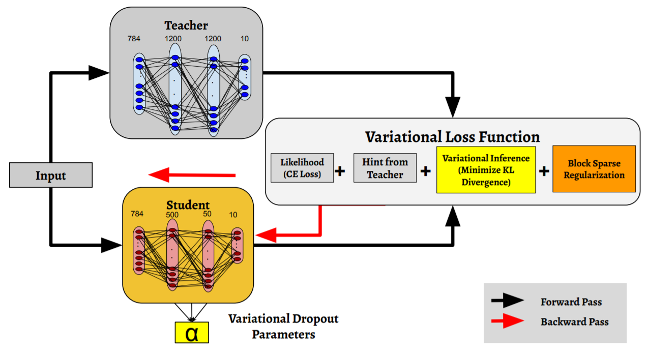
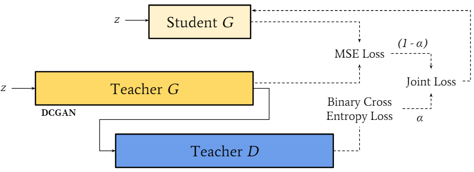
\subsection{Generative Modelling Based Model Distillation} Here, we describe how two commonly used generative models, variational inference (VI) and generative adversarial networks (GANs), have been applied to learning a student networks.

Variational Inference Learned Student

Distilling SimCLR

~\citet{chen2020big} shows that an unsupervised learned constrastive-based CNN requires 10 times less labels to for fine-tuning on ImageNet compared to only using a supervised contrastive CNN (ResNet architecture). They find a strong correlation between the size of the pretrained network and the amount of labels it requires for fine-tuning. Finally, the constrastive network is distilled into a smaller version without sacrificing little classification accuracy.

Relational Model Distillation

~\citet{park2019relational} apply knowledge distillation to relational data and propose distance (huber) and angular-based (cosine proximity) loss functions that account for different relational structures and claim that metric learning allows the student relational network to outperform the teacher network on achieving SoTA on relational datasets.

</div>

The \(\psi(\cdot)\) similarity function from the relation teacher network outputs a score that is transferred to as a pseudo target for the teacher network to learn from as,

In the case of the angular loss shown in \autoref{eq:ang_loss}, \(\vec{e}^{ij} = \frac{t_i - t_j}{|| t_i - t_j ||_2}$, $e^{kj} = \frac{t_k - t_j}{ ||t_k - t_{j}||^2}\).

They find that measuring the angle between teacher and student outputs as input to the huber loss \(\mathcal{L}_{delta}\) leads to improved performance when compared to previous SoTA on metric learning tasks.

This is then used as a regularization terms to the task specific loss as, \(\begin{equation}\label{eq:total_loss} \mathcal{L}_{\text{task}} + \lambda_{\text{MD}} \mathcal{L}_{MD} \end{equation}\)

When used in metric learning the triplet loss shown in \autoref{eq:triplet_loss} is used.

\autoref{fig:recall_rd} shows the test data recall @1 on tested relational datasets. The teacher network is trained with the triplet loss and student distils the knowledge using \autoref{eq:total_loss}. Left of the dashed line are results on the training domain while on the right shows results on the remaining domains.

Correlation Congruence Model Distillation

~\citet{peng2019correlation} Most teacher-student frameworks based on knowledge distillation (KD) depend on a strong congruent constraint on instance level. However, they usually ignore the correlation between multiple instances, which is also valuable for knowledge transfer. In this work, we propose a new frame-work named correlation congruence for knowledge distillation (CCKD), which transfers not only the instance-level information but also the correlation between instances. Furthermore, a generalized kernel method based on Taylor series expansion is proposed to better capture the correlation between instances. Empirical experiments and ablation studies on image classification tasks (including CIFAR-100, ImageNet-1K) and metric learning tasks (including ReID and Face Recognition) show that the proposed CCKD substantially outperforms the original KD and other SOTA KD-based methods. The CCKD can be easily deployed in the majority of the teacher-student framework such as KD and hint-based learning methods.

Layer Transfer in Model Distillation

~\citet{yim2017gift} We introduce a novel technique for knowledge transfer,where knowledge from a pretrained deep neural network (DNN) is distilled and transferred to another DNN. As the DNN maps from the input space to the output space through many layers sequentially, we define the distilled knowledge to be transferred in terms of flow between layers, which is calculated by computing the inner product between features from two layers. When we compare the student DNN and the original network with the same size as the student DNN but trained without a teacher network, the proposed method of transferring the distilled knowledge as the flow between two layers exhibits three important phenomena: (1) the student DNN that learns the distilled knowledge is optimized much faster than the original model; (2) the student DNN outperforms the original DNN; and (3) the student DNN can learn the distilled knowledge from a teacher DNN that is trained at a different task, and the student DNN outperforms the original DNN that is trained from scratch.

Knowledge Distillation via Factor Transfer

~\citet{kim2018paraphrasing} Many researchers have sought ways of model compression to reduce the size of a deep neural network (DNN) with minimal performance degradation in order to use DNNs in embedded systems. Among the model compression methods, a method called knowledge transfer is to train a student network with a stronger teacher network. In this paper, we propose a novel knowledge transfer method which uses convolutional operations to paraphrase teacher's knowledge and to translate it for the student. This is done by two convolutional modules, which are called a paraphraser and a translator. The paraphraser is trained in an unsupervised manner to extract the teacher factors which are defined as paraphrased information of the teacher network. The translator located at the student network extracts the student factors and helps to translate the teacher factors by mimicking them. We observed that our student network trained with the proposed factor transfer method outperforms the ones trained with conventional knowledge transfer methods.

Attention-Transfer Model Distillation

~\citet{song2018neural} use attention-based knowledge distillation for fashion matching that jointly learns to match clothing items while incorporating domain knowledge rules defined by clothing description where the attention learns to assign weights corresponding to the rule confidence.

Variational Information Model Distillation

~\citet{ahn2019variational} Transferring knowledge from a teacher neural network pretrained on the same or a similar task to a student neural network can significantly improve the performance of the student neural network. Existing knowledge transfer approaches match the activations or the corresponding hand-crafted features of the teacher and the student networks. We propose an information-theoretic framework for knowledge transfer which formulates knowledge transfer as maximizing the mutual information between the teacher and the student networks. We compare our method with existing knowledge transfer methods on both knowledge distillation and transfer learning tasks and show that our method consistently outperforms existing methods. We further demon-strate the strength of our method on knowledge transfer across heterogeneous network architectures by transferring knowledge from a convolutional neural network (CNN) to a multi-layer perceptron (MLP) on CIFAR-10. The resulting MLP significantly outperforms the SoTA methods and it achieves similar performance to the CNN with a single convolutional layer.

Data-Free Model Distillation

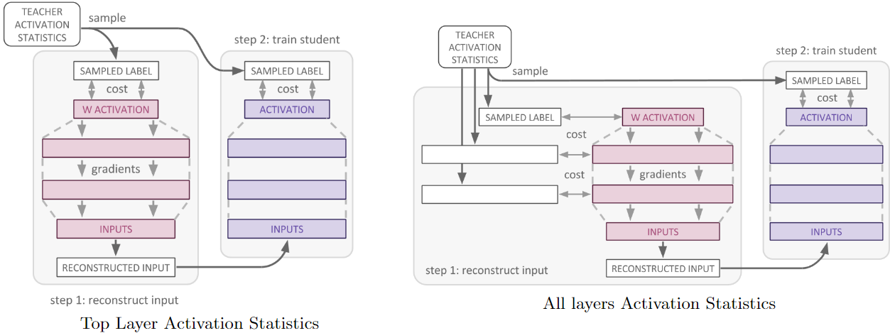
~\citet{lopes2017data} aim to distill in the scenario where it is not possible to have access to the original data the teacher network was trained on. This can occur due to privacy issues (e.g personal medical data, models trained case-based legal data) or the data is no longer available or some way corrupted. They store the sufficient statistics (e.g mean and covariance) of activation outputs from the original data along with the pretrained teacher network to reconstruct the original training data input. This is achieved by trying to find images that have the highest representational similarity to those given by the representations from the activation records of the teacher network. Gaussian noise is passed as input to the teacher and update gradients to the noise to minimize the difference between the recorded activation outputs and those of the noisy image and repeat this to reconstruct the teachers view of the original data.

The left figure in \autoref{fig:data_free_md} shows the activation statistics for the top layer and a sample drawn that is used to optimize the input to teacher network to reconstruct the activations. The reconstructed input is then fed to the student network. On the right, the same procedure follows but for reconstructing activations for all layers of the teacher network.

</div>

They manage to compress the teacher network to half the size in the student network using the reconstructed inputs constructed from using the metadata. The amount of compression achieved is contingent on the quality of the metadata, in their case they only used activation statistics. We posit that the notion of creating synthetic data from summary statistics of the original data to train the student network is worth further investigation.

Dataset Distillation

Instead of reducing the size of the model,~\citeauthor{wang2018dataset} have proposed to distill thousands of images into a small number of distilled images (e.g) and training on the distilled set of images to achieve similar performance to a model trained on all raw images. Unike previous approaches, this data augmentation process does not restrict the reduced image set to be real and hence have the flexbility to produce compact highly informative images although they are non-interpretable.

• Get a minibatch of real training data \(\vec{x}_t = \{xt,j\}^n_{j=1}\)
• Sample a batch of initial weights \(\theta^{(j)}_0 \sim p(\theta_0)\)
• for each sampled \(\theta^(j)_0\) do
  • Compute updated parameter with GD: \(\theta^(j)_1 = \theta^{(j)}_0 − \tilde{\eta}\nabla_{\theta^{(j)}_0} (\tilde{\vec{x}}, \theta^{(j)}_0)\)
  • Evaluate the objective function on real training data: \(\mathcal{L}^{(j)} = \ell(\vec{x}_t, \mathbf{\theta}^{(j)}_1)\)
  • end for
• Update \(\tilde{\vec{x}} ← \tilde{\vec{x}} − \alpha \nabla_{\tilde{x}} P j L^{(j)}\), and \(\tilde{\eta} ← \tilde{\eta} - \alpha \nabla \tilde{\eta} Pj L^{(j)}\)

Similar to our approach, data-free knowledge distillation also optimizes synthetic data samples, but with a different objective of matching activation statistics of a teacher model in knowledge distillation (Lopes et al., 2017). Our method is also related to the theoretical concept of teaching dimension, which specifies the size of dataset necessary to teach a target model to a learner (Shinohara & Miyano, 1991; Goldman & Kearns, 1995). However, methods (Zhu, 2013; 2015) inspired by this concept need the existence of target models, which our method does not require.

Instead of distilling the knowledge from a teacher network, dataset distillation~\cite{wang2018dataset} distills a training set of input images into a single image per class and reach performance close to that of an equivalent model trained using all the original training data. Although, the distilled images for each class are unrecognizable to a human, the learning algorithm is able to approximate the original data on MNIST (60k training images) and CIFAR-10 (50k training images) in only a few gradient steps.

Standard training usually applies minibatch stochastic gradient descent or its variants. At each step \(t\), a minibatch of training data \(x_t = \{\vec{x}_{t,j}\}_{j=1}^n\) is sampled to update the current parameters as

where \(\eta\) is the learning rate. Such a training process often takes tens of thousands or even millions of update steps to converge. Instead, we aim to learn a tiny set of synthetic distilled training data \(\tilde{x} = \{\tilde{\vec{x}}_i\}_{i=1}^{M}\) with $M « N$ and a corresponding learning rate $\tilde{\eta}$ so that a single gradient descent step such as

using these learned synthetic data $\tilde{\vec{x}}$ can greatly boost the performance on the real test set. Given an initial $\mathbf{\theta}_0$, we obtain these synthetic data $\tilde{\vec{x}}$ and learning rate $\tilde{\eta}$ by minimizing the objective below \(\mathcal{L}\)

where we derive the new weights $\mathbf{\theta}_1$ as a function of distilled data $\tilde{x}$ and learning rate $\tilde{\eta}$ using Equation 2 and then evaluate the new weights over all the training data $x$. The loss $L(\tilde{x}, \tilde{\eta}; \mathbf{\theta}_0)$ is differentiable w.r.t. $\tilde{x}$ and $\tilde{\eta}$, and can thus be optimized using standard gradient-based methods. In many classification tasks, the data $x$ may contain discrete parts, e.g., class labels in data-label pairs. For such cases, we fix the discrete parts rather than learn them.